# load dslabs package
library("dslabs")Data Analysis intro
Introduction
In this exercise we will use the gapminder dataset from the dslabs package
Required Packages
This exercise uses the following packages:
- dslabs: provides the gapminder dataset
- dplyr: data wrangling (filter/select)
- ggplot2: plotting
- broom: tidy outputs from linear models
Load all packages at the top of the analysis so they are available later.
Each library () call attaches one package.
library(dslabs) # provides the gapminder dataset
library(dplyr) # used for filtering/selecting columns
library(ggplot2) # used for plotting
library(broom) # used to tidy lm() results
Loading and Checking the data
# help(gapminder)
# get an overview of data structure
str(gapminder)
'data.frame': 10545 obs. of 9 variables:
$ country : Factor w/ 185 levels "Albania","Algeria",..: 1 2 3 4 5 6 7 8 9 10 ...
$ year : int 1960 1960 1960 1960 1960 1960 1960 1960 1960 1960 ...
$ infant_mortality: num 115.4 148.2 208 NA 59.9 ...
$ life_expectancy : num 62.9 47.5 36 63 65.4 ...
$ fertility : num 6.19 7.65 7.32 4.43 3.11 4.55 4.82 3.45 2.7 5.57 ...
$ population : num 1636054 11124892 5270844 54681 20619075 ...
$ gdp : num NA 1.38e+10 NA NA 1.08e+11 ...
$ continent : Factor w/ 5 levels "Africa","Americas",..: 4 1 1 2 2 3 2 5 4 3 ...
$ region : Factor w/ 22 levels "Australia and New Zealand",..: 19 11 10 2 15 21 2 1 22 21 ...# get a summary of data
summary(gapminder) country year infant_mortality life_expectancy
Albania : 57 Min. :1960 Min. : 1.50 Min. :13.20
Algeria : 57 1st Qu.:1974 1st Qu.: 16.00 1st Qu.:57.50
Angola : 57 Median :1988 Median : 41.50 Median :67.54
Antigua and Barbuda: 57 Mean :1988 Mean : 55.31 Mean :64.81
Argentina : 57 3rd Qu.:2002 3rd Qu.: 85.10 3rd Qu.:73.00
Armenia : 57 Max. :2016 Max. :276.90 Max. :83.90
(Other) :10203 NA's :1453
fertility population gdp continent
Min. :0.840 Min. :3.124e+04 Min. :4.040e+07 Africa :2907
1st Qu.:2.200 1st Qu.:1.333e+06 1st Qu.:1.846e+09 Americas:2052
Median :3.750 Median :5.009e+06 Median :7.794e+09 Asia :2679
Mean :4.084 Mean :2.701e+07 Mean :1.480e+11 Europe :2223
3rd Qu.:6.000 3rd Qu.:1.523e+07 3rd Qu.:5.540e+10 Oceania : 684
Max. :9.220 Max. :1.376e+09 Max. :1.174e+13
NA's :187 NA's :185 NA's :2972
region
Western Asia :1026
Eastern Africa : 912
Western Africa : 912
Caribbean : 741
South America : 684
Southern Europe: 684
(Other) :5586 # determine the type of object gapminder is
class(gapminder)[1] "data.frame"Processing data
# Create a new object that keeps ONLY rows where continent == "Africa"
# (this subsets the original gapminder data frame)
africadata <- gapminder[gapminder$continent == "Africa", ]

# Check the structure of the new Africa-only dataset
str(africadata)
'data.frame': 2907 obs. of 9 variables:
$ country : Factor w/ 185 levels "Albania","Algeria",..: 2 3 18 22 26 27 29 31 32 33 ...
$ year : int 1960 1960 1960 1960 1960 1960 1960 1960 1960 1960 ...
$ infant_mortality: num 148 208 187 116 161 ...
$ life_expectancy : num 47.5 36 38.3 50.3 35.2 ...
$ fertility : num 7.65 7.32 6.28 6.62 6.29 6.95 5.65 6.89 5.84 6.25 ...
$ population : num 11124892 5270844 2431620 524029 4829291 ...
$ gdp : num 1.38e+10 NA 6.22e+08 1.24e+08 5.97e+08 ...
$ continent : Factor w/ 5 levels "Africa","Americas",..: 1 1 1 1 1 1 1 1 1 1 ...
$ region : Factor w/ 22 levels "Australia and New Zealand",..: 11 10 20 17 20 5 10 20 10 10 ...# Get summary statistics for the Africa-only dataset
summary(africadata) country year infant_mortality life_expectancy
Algeria : 57 Min. :1960 Min. : 11.40 Min. :13.20
Angola : 57 1st Qu.:1974 1st Qu.: 62.20 1st Qu.:48.23
Benin : 57 Median :1988 Median : 93.40 Median :53.98
Botswana : 57 Mean :1988 Mean : 95.12 Mean :54.38
Burkina Faso: 57 3rd Qu.:2002 3rd Qu.:124.70 3rd Qu.:60.10
Burundi : 57 Max. :2016 Max. :237.40 Max. :77.60
(Other) :2565 NA's :226
fertility population gdp continent
Min. :1.500 Min. : 41538 Min. :4.659e+07 Africa :2907
1st Qu.:5.160 1st Qu.: 1605232 1st Qu.:8.373e+08 Americas: 0
Median :6.160 Median : 5570982 Median :2.448e+09 Asia : 0
Mean :5.851 Mean : 12235961 Mean :9.346e+09 Europe : 0
3rd Qu.:6.860 3rd Qu.: 13888152 3rd Qu.:6.552e+09 Oceania : 0
Max. :8.450 Max. :182201962 Max. :1.935e+11
NA's :51 NA's :51 NA's :637
region
Eastern Africa :912
Western Africa :912
Middle Africa :456
Northern Africa :342
Southern Africa :285
Australia and New Zealand: 0
(Other) : 0 library(dplyr)
Attaching package: 'dplyr'The following objects are masked from 'package:stats':
filter, lagThe following objects are masked from 'package:base':
intersect, setdiff, setequal, union# Infant mortality vs life expectancy
africa_im_le <- africadata %>%
select(infant_mortality, life_expectancy)
str(africa_im_le)'data.frame': 2907 obs. of 2 variables:
$ infant_mortality: num 148 208 187 116 161 ...
$ life_expectancy : num 47.5 36 38.3 50.3 35.2 ...summary(africa_im_le) infant_mortality life_expectancy
Min. : 11.40 Min. :13.20
1st Qu.: 62.20 1st Qu.:48.23
Median : 93.40 Median :53.98
Mean : 95.12 Mean :54.38
3rd Qu.:124.70 3rd Qu.:60.10
Max. :237.40 Max. :77.60
NA's :226 # Population vs life expectancy
africa_pop_le <- africadata %>%
select(population, life_expectancy)
str(africa_pop_le)'data.frame': 2907 obs. of 2 variables:
$ population : num 11124892 5270844 2431620 524029 4829291 ...
$ life_expectancy: num 47.5 36 38.3 50.3 35.2 ...summary(africa_pop_le) population life_expectancy
Min. : 41538 Min. :13.20
1st Qu.: 1605232 1st Qu.:48.23
Median : 5570982 Median :53.98
Mean : 12235961 Mean :54.38
3rd Qu.: 13888152 3rd Qu.:60.10
Max. :182201962 Max. :77.60
NA's :51 Plotting
Making plots for each of the new subsets.
# load ggplot2 here since we will make plots

library(ggplot2)
# Plot life expectancy as a function of infant mortality
ggplot(africa_im_le, aes(x = infant_mortality, y = life_expectancy)) +
geom_point()Warning: Removed 226 rows containing missing values or values outside the scale range
(`geom_point()`).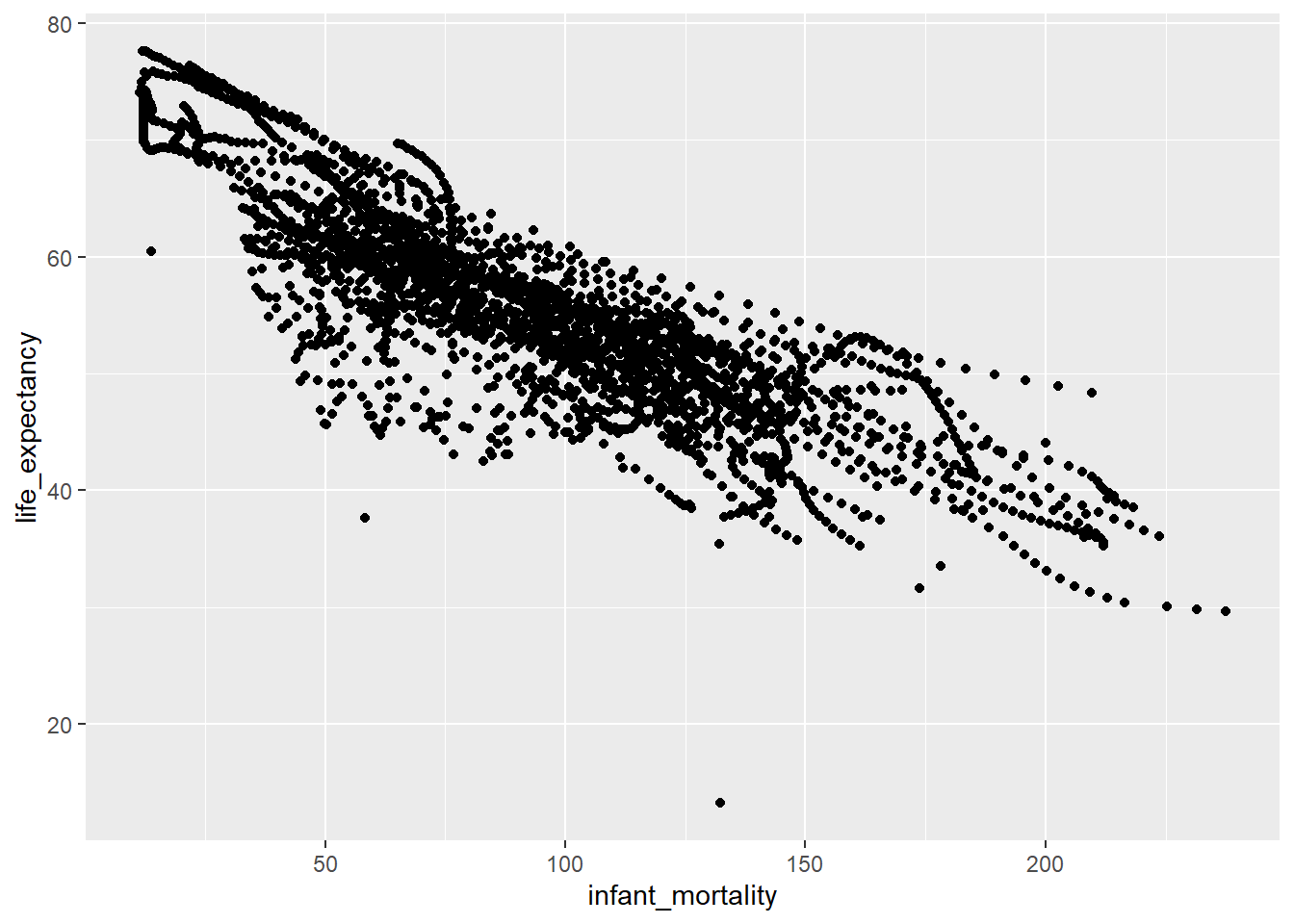
# Plot life expectancy as a function of population size (log scale)

ggplot(africa_pop_le, aes(x = population, y = life_expectancy)) +
geom_point() +
scale_x_log10()
Warning: Removed 51 rows containing missing values or values outside the scale range
(`geom_point()`).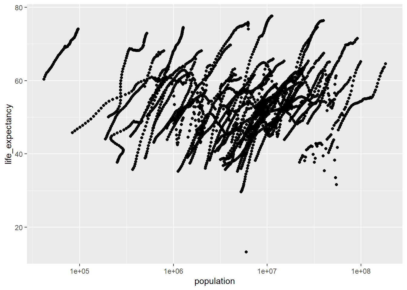
More data processing
To understand which years have missing infant mortality data, we first check which years contain NA values for infant_mortality. Then we select a year with complete data.
# Find rows with missing infant mortality

africa_na <- africadata %>%
filter(is.na(infant_mortality))

# Check which years have missing values

table(africa_na$year)
1960 1961 1962 1963 1964 1965 1966 1967 1968 1969 1970 1971 1972 1973 1974 1975
  10   17   16   16   15   14   13   11   11    7    5    6    6    6    5    5
1976 1977 1978 1979 1980 1981 2016
   3    3    2    2    1    1   51
# Keep only data from the year 2000
africa_2000 <- africadata %>%
filter(year == 2000)
# Check structure and summary
str(africa_2000)'data.frame': 51 obs. of 9 variables:
$ country : Factor w/ 185 levels "Albania","Algeria",..: 2 3 18 22 26 27 29 31 32 33 ...
$ year : int 2000 2000 2000 2000 2000 2000 2000 2000 2000 2000 ...
$ infant_mortality: num 33.9 128.3 89.3 52.4 96.2 ...
$ life_expectancy : num 73.3 52.3 57.2 47.6 52.6 46.7 54.3 68.4 45.3 51.5 ...
$ fertility : num 2.51 6.84 5.98 3.41 6.59 7.06 5.62 3.7 5.45 7.35 ...
$ population : num 31183658 15058638 6949366 1736579 11607944 ...
$ gdp : num 5.48e+10 9.13e+09 2.25e+09 5.63e+09 2.61e+09 ...
$ continent : Factor w/ 5 levels "Africa","Americas",..: 1 1 1 1 1 1 1 1 1 1 ...
$ region : Factor w/ 22 levels "Australia and New Zealand",..: 11 10 20 17 20 5 10 20 10 10 ...summary(africa_2000) country year infant_mortality life_expectancy
Algeria : 1 Min. :2000 Min. : 12.30 Min. :37.60
Angola : 1 1st Qu.:2000 1st Qu.: 60.80 1st Qu.:51.75
Benin : 1 Median :2000 Median : 80.30 Median :54.30
Botswana : 1 Mean :2000 Mean : 78.93 Mean :56.36
Burkina Faso: 1 3rd Qu.:2000 3rd Qu.:103.30 3rd Qu.:60.00
Burundi : 1 Max. :2000 Max. :143.30 Max. :75.00
(Other) :45
fertility population gdp continent
Min. :1.990 Min. : 81154 Min. :2.019e+08 Africa :51
1st Qu.:4.150 1st Qu.: 2304687 1st Qu.:1.274e+09 Americas: 0
Median :5.550 Median : 8799165 Median :3.238e+09 Asia : 0
Mean :5.156 Mean : 15659800 Mean :1.155e+10 Europe : 0
3rd Qu.:5.960 3rd Qu.: 17391242 3rd Qu.:8.654e+09 Oceania : 0
Max. :7.730 Max. :122876723 Max. :1.329e+11
region
Eastern Africa :16
Western Africa :16
Middle Africa : 8
Northern Africa : 6
Southern Africa : 5
Australia and New Zealand: 0
(Other) : 0 More Plotting
We now repeat the same plots as before, but only using data from the year 2000.
# Create 2000-only versions of the two 2-column datasets

africa2000_im_le <- africa_2000 %>%
  select(infant_mortality, life_expectancy)


str(africa2000_im_le)
'data.frame': 51 obs. of 2 variables:
$ infant_mortality: num 33.9 128.3 89.3 52.4 96.2 ...
$ life_expectancy : num 73.3 52.3 57.2 47.6 52.6 46.7 54.3 68.4 45.3 51.5 ...#summary of infant mortality and life expectancy data in 2000
summary(africa2000_im_le) infant_mortality life_expectancy
Min. : 12.30 Min. :37.60
1st Qu.: 60.80 1st Qu.:51.75
Median : 80.30 Median :54.30
Mean : 78.93 Mean :56.36
3rd Qu.:103.30 3rd Qu.:60.00
Max. :143.30 Max. :75.00 africa2000_pop_le <- africa_2000 %>%
select(population, life_expectancy)
str(africa2000_pop_le)'data.frame': 51 obs. of 2 variables:
$ population : num 31183658 15058638 6949366 1736579 11607944 ...
$ life_expectancy: num 73.3 52.3 57.2 47.6 52.6 46.7 54.3 68.4 45.3 51.5 ...#summary of population and life expectancy data in 2000
summary(africa2000_pop_le) population life_expectancy
Min. : 81154 Min. :37.60
1st Qu.: 2304687 1st Qu.:51.75
Median : 8799165 Median :54.30
Mean : 15659800 Mean :56.36
3rd Qu.: 17391242 3rd Qu.:60.00
Max. :122876723 Max. :75.00 ggplot(africa_2000, aes(x = infant_mortality, y = life_expectancy)) +
geom_point()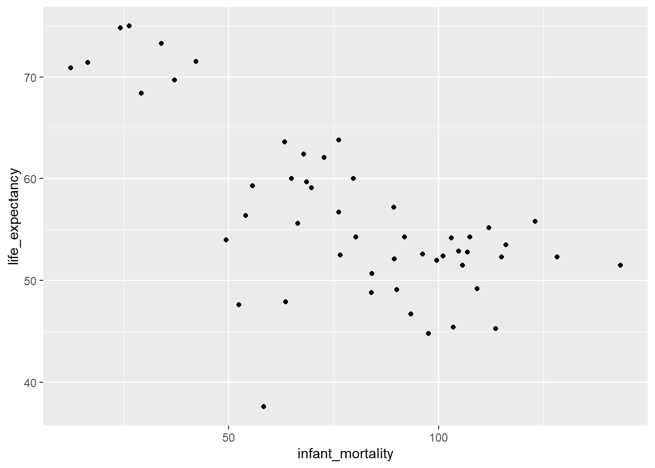
ggplot(africa_2000, aes(x = population, y = life_expectancy)) +
geom_point() +
scale_x_log10()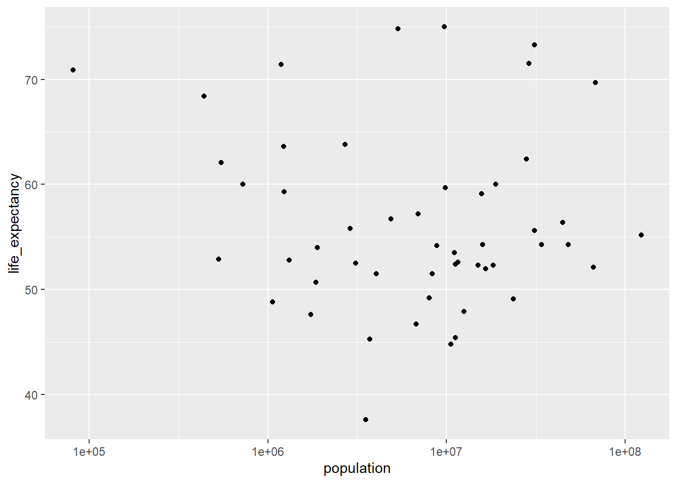
A simple fit
We fit linear regression models using life expectancy as the response variable and infant mortality and population size as separate predictors, based on the Africa-only data from the year 2000.
# Fit 1: linear model with life expectancy as outcome and infant mortality as predictor (year 2000 only)

fit1 <- lm(life_expectancy ~ infant_mortality, data = africa_2000)

# Show model results

summary(fit1)
Call:
lm(formula = life_expectancy ~ infant_mortality, data = africa_2000)

Residuals:
     Min       1Q   Median       3Q      Max
-22.6651  -3.7087   0.9914   4.0408   8.6817

Coefficients:
                 Estimate Std. Error t value Pr(>|t|)
(Intercept)      71.29331    2.42611  29.386  < 2e-16 ***
infant_mortality -0.18916    0.02869  -6.594 2.83e-08 ***
---
Signif. codes:  0 '***' 0.001 '**' 0.01 '*' 0.05 '.' 0.1 ' ' 1

Residual standard error: 6.221 on 49 degrees of freedom
Multiple R-squared:  0.4701,    Adjusted R-squared:  0.4593
F-statistic: 43.48 on 1 and 49 DF,  p-value: 2.826e-08
# Fit 2: linear model with life expectancy as outcome and population as predictor (year 2000 only)
fit2 <- lm(life_expectancy ~ population, data = africa_2000)
# Show model results
summary(fit2)
Call:
lm(formula = life_expectancy ~ population, data = africa_2000)

Residuals:
    Min      1Q  Median      3Q     Max
-18.429  -4.602  -2.568   3.800  18.802

Coefficients:
             Estimate Std. Error t value Pr(>|t|)
(Intercept) 5.593e+01  1.468e+00  38.097   <2e-16 ***
population  2.756e-08  5.459e-08   0.505    0.616
---
Signif. codes:  0 '***' 0.001 '**' 0.01 '*' 0.05 '.' 0.1 ' ' 1

Residual standard error: 8.524 on 49 degrees of freedom
Multiple R-squared:  0.005176,  Adjusted R-squared:  -0.01513
F-statistic: 0.2549 on 1 and 49 DF,  p-value: 0.6159
This section contribution by Austin_Hill
#Load in dslabs
library(dslabs)
#look at data
str(death_prob)'data.frame': 240 obs. of 3 variables:
$ age : int 0 1 2 3 4 5 6 7 8 9 ...
$ sex : Factor w/ 2 levels "Female","Male": 2 2 2 2 2 2 2 2 2 2 ...
$ prob: num 0.006383 0.000453 0.000282 0.00023 0.000169 ...summary(death_prob) age sex prob
Min. : 0.00 Female:120 Min. :0.000091
1st Qu.: 29.75 Male :120 1st Qu.:0.001318
Median : 59.50 Median :0.008412
Mean : 59.50 Mean :0.127254
3rd Qu.: 89.25 3rd Qu.:0.138332
Max. :119.00 Max. :0.899639 #Type of class the data is
class(death_prob)[1] "data.frame"# add dplyr package
library(dplyr)# Filter data to only females of the age of 16 +
femaledata16 <- death_prob %>%
filter(sex == "Female", age >= 16)
# look at femaledata
str(femaledata16)'data.frame': 104 obs. of 3 variables:
$ age : int 16 17 18 19 20 21 22 23 24 25 ...
$ sex : Factor w/ 2 levels "Female","Male": 1 1 1 1 1 1 1 1 1 1 ...
$ prob: num 0.000254 0.000294 0.00033 0.000364 0.000399 0.000436 0.000469 0.000497 0.000522 0.000546 ...summary(femaledata16) age sex prob
Min. : 16.00 Female:104 Min. :0.000254
1st Qu.: 41.75 Male : 0 1st Qu.:0.001541
Median : 67.50 Median :0.012245
Mean : 67.50 Mean :0.140093
3rd Qu.: 93.25 3rd Qu.:0.186705
Max. :119.00 Max. :0.899639 # add ggplot
library(ggplot2)# plotting 16+ girls probability of death in the next year in the USA in 2015
ggplot(femaledata16, aes(x = age, y = prob)) +
geom_line() +
geom_point() +
labs(
title = "Probability of death vs Age (Females)",
x = "Age",
y = "Probability"
) +
theme_minimal()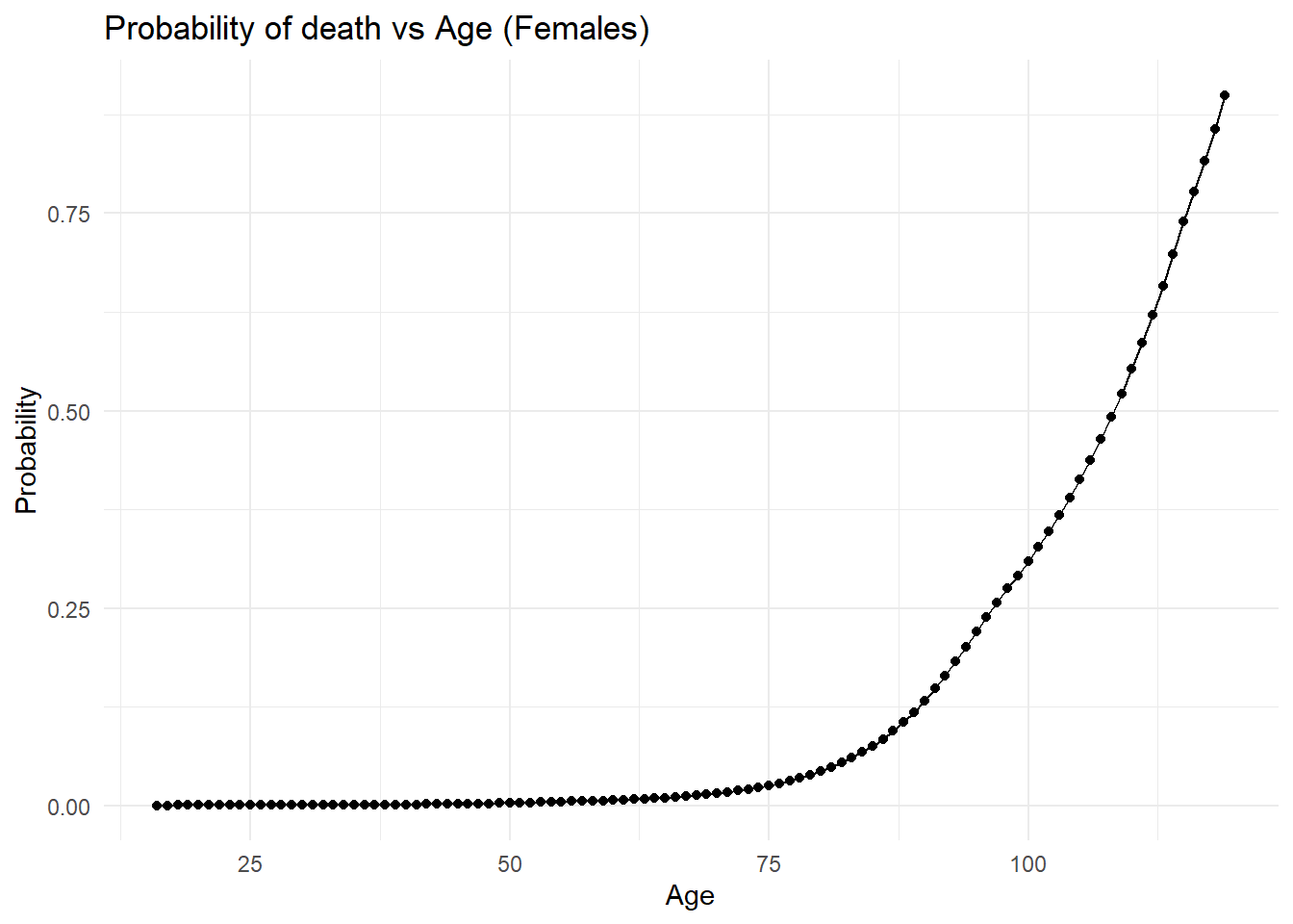
# Filter data to only males of the age of 16 +
maledata16 <- death_prob %>%
  filter(sex == "Male", age >= 16)
# look at femaledata
str(maledata16)
'data.frame': 104 obs. of 3 variables:
$ age : int 16 17 18 19 20 21 22 23 24 25 ...
$ sex : Factor w/ 2 levels "Female","Male": 2 2 2 2 2 2 2 2 2 2 ...
$ prob: num 0.00053 0.000655 0.000791 0.000934 0.001085 ...summary(maledata16) age sex prob
Min. : 16.00 Female: 0 Min. :0.000530
1st Qu.: 41.75 Male :104 1st Qu.:0.002472
Median : 67.50 Median :0.019114
Mean : 67.50 Mean :0.153407
3rd Qu.: 93.25 3rd Qu.:0.228207
Max. :119.00 Max. :0.899639 # plotting 16+ males probability of death in the next year in the USA in 2015
ggplot(maledata16, aes(x = age, y = prob)) +
geom_line() +
geom_point() +
labs(
title = "Probability of death vs Age (Males)",
x = "Age",
y = "Probability"
) +
theme_minimal()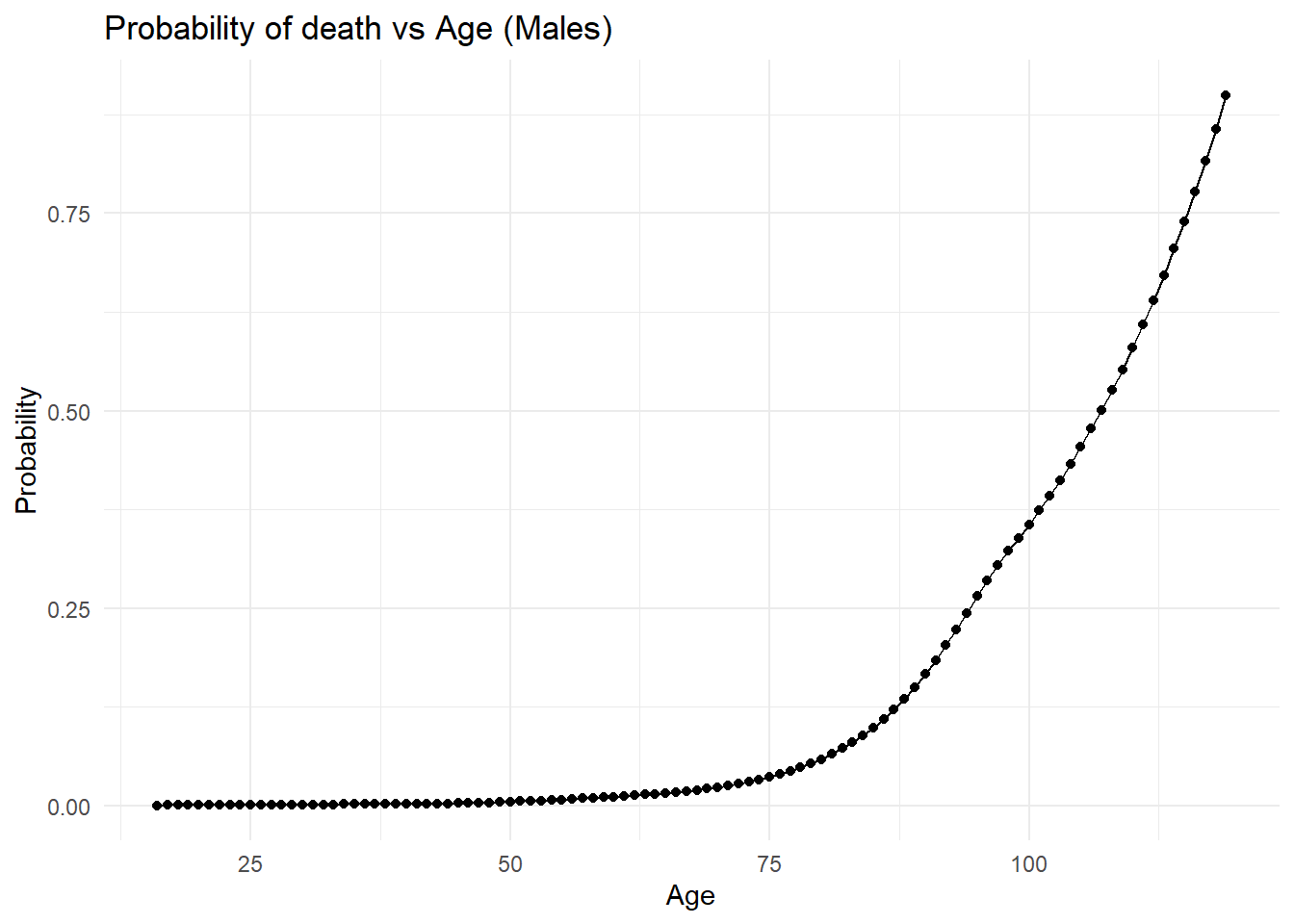
# Compare females and males 16+ for significant differnces in the data combined
combined <- rbind(femaledata16, maledata16)

model1 <- lm(prob ~ age + sex, data = combined)
summary(model1)
Call:
lm(formula = prob ~ age + sex, data = combined)

Residuals:
     Min       1Q   Median       3Q      Max
-0.17611 -0.12053 -0.02084  0.09396  0.43905

Coefficients:
              Estimate Std. Error t value Pr(>|t|)
(Intercept) -0.2799717  0.0259728 -10.779   <2e-16 ***
age          0.0062232  0.0003257  19.106   <2e-16 ***
sexMale      0.0133138  0.0195563   0.681    0.497
---
Signif. codes:  0 '***' 0.001 '**' 0.01 '*' 0.05 '.' 0.1 ' ' 1

Residual standard error: 0.141 on 205 degrees of freedom
Multiple R-squared:  0.6407,    Adjusted R-squared:  0.6372
F-statistic: 182.8 on 2 and 205 DF,  p-value: < 2.2e-16