Fitting Exercise

Loading and Checking the data

The raw dataset contains repeated time‐series measurements of drug concentration (DV) over time (TIME) for each individual (ID). The data also includes dosing information (DOSE, AMT) and basic demographics (AGE, SEX, RACE WT, HT).

library(tidyverse)

── Attaching core tidyverse packages ──────────────────────── tidyverse 2.0.0 ──
✔ dplyr     1.2.0     ✔ readr     2.1.6
✔ forcats   1.0.1     ✔ stringr   1.6.0
✔ ggplot2   4.0.1     ✔ tibble    3.3.1
✔ lubridate 1.9.5     ✔ tidyr     1.3.2
✔ purrr     1.2.1     
── Conflicts ────────────────────────────────────────── tidyverse_conflicts() ──
✖ dplyr::filter() masks stats::filter()
✖ dplyr::lag()    masks stats::lag()
ℹ Use the conflicted package (<http://conflicted.r-lib.org/>) to force all conflicts to become errors

library(here)

here() starts at C:/Users/PC/Documents/GitHub/SaraaAljawad-portfolio

dat_raw <- read_csv(here("fitting-exercise","Mavoglurant_A2121_nmpk.csv"))

Rows: 2678 Columns: 17
── Column specification ────────────────────────────────────────────────────────
Delimiter: ","
dbl (17): ID, CMT, EVID, EVI2, MDV, DV, LNDV, AMT, TIME, DOSE, OCC, RATE, AG...

ℹ Use `spec()` to retrieve the full column specification for this data.
ℹ Specify the column types or set `show_col_types = FALSE` to quiet this message.

dim(dat_raw)

[1] 2678   17

head(dat_raw)

# A tibble: 6 × 17
     ID   CMT  EVID  EVI2   MDV    DV  LNDV   AMT  TIME  DOSE   OCC  RATE   AGE
  <dbl> <dbl> <dbl> <dbl> <dbl> <dbl> <dbl> <dbl> <dbl> <dbl> <dbl> <dbl> <dbl>
1   793     1     1     1     1     0  0       25 0        25     1    75    42
2   793     2     0     0     0   491  6.20     0 0.2      25     1     0    42
3   793     2     0     0     0   605  6.40     0 0.25     25     1     0    42
4   793     2     0     0     0   556  6.32     0 0.367    25     1     0    42
5   793     2     0     0     0   310  5.74     0 0.533    25     1     0    42
6   793     2     0     0     0   237  5.47     0 0.7      25     1     0    42
# ℹ 4 more variables: SEX <dbl>, RACE <dbl>, WT <dbl>, HT <dbl>

Quick plot of concentration over time

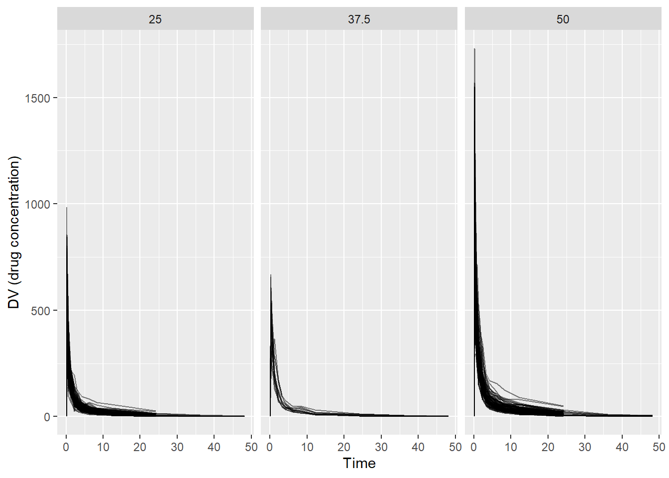
ggplot(dat_raw, aes(x = TIME, y = DV, group = ID)) +
  geom_line(alpha = 0.5) +
  facet_wrap(~ DOSE) +
  labs(
    x = "Time",
    y = "DV (drug concentration)"
  )

Plotting DV versus TIME (grouped by ID and stratified by DOSE): concentrations are highest shortly after dosing and decline over time. Higher dose groups appear to have higher concentration curves overall.

Remove OCC = 2

dat1 <- dat_raw %>%
  filter(OCC == 1)

dim(dat1)

[1] 1665   17

table(dat_raw$OCC)

   1    2 
1665 1013 

Some individuals have multiple occasions (OCC=1 and OCC=2), indicating repeated dosing/measurement periods. To keep the exercise simple and avoid having multiple trajectories per person, I kept only OCC=1 and removed OCC=2.

Compute total drug amount per individual (Y)

y_df <- dat1 %>%
  filter(TIME != 0) %>%
  group_by(ID) %>%
  summarize(Y = sum(DV, na.rm = TRUE))

dim(y_df)

[1] 120   2

head(y_df)

# A tibble: 6 × 2
     ID     Y
  <dbl> <dbl>
1   793 2691.
2   794 2639.
3   795 2150.
4   796 1789.
5   797 3126.
6   798 2337.

Extract baseline rows (TIME = 0)

base_df <- dat1 %>%
  filter(TIME == 0)

dim(base_df)

[1] 120  17

head(base_df)

# A tibble: 6 × 17
     ID   CMT  EVID  EVI2   MDV    DV  LNDV   AMT  TIME  DOSE   OCC  RATE   AGE
  <dbl> <dbl> <dbl> <dbl> <dbl> <dbl> <dbl> <dbl> <dbl> <dbl> <dbl> <dbl> <dbl>
1   793     1     1     1     1     0     0    25     0    25     1    75    42
2   794     1     1     1     1     0     0    25     0    25     1   150    24
3   795     1     1     1     1     0     0    25     0    25     1   150    31
4   796     1     1     1     1     0     0    25     0    25     1   150    46
5   797     1     1     1     1     0     0    25     0    25     1   150    41
6   798     1     1     1     1     0     0    25     0    25     1   150    27
# ℹ 4 more variables: SEX <dbl>, RACE <dbl>, WT <dbl>, HT <dbl>

Join baseline data with total drug (Y)

dat_person <- base_df %>%
  left_join(y_df, by = "ID")

dim(dat_person)

[1] 120  18

head(dat_person)

# A tibble: 6 × 18
     ID   CMT  EVID  EVI2   MDV    DV  LNDV   AMT  TIME  DOSE   OCC  RATE   AGE
  <dbl> <dbl> <dbl> <dbl> <dbl> <dbl> <dbl> <dbl> <dbl> <dbl> <dbl> <dbl> <dbl>
1   793     1     1     1     1     0     0    25     0    25     1    75    42
2   794     1     1     1     1     0     0    25     0    25     1   150    24
3   795     1     1     1     1     0     0    25     0    25     1   150    31
4   796     1     1     1     1     0     0    25     0    25     1   150    46
5   797     1     1     1     1     0     0    25     0    25     1   150    41
6   798     1     1     1     1     0     0    25     0    25     1   150    27
# ℹ 5 more variables: SEX <dbl>, RACE <dbl>, WT <dbl>, HT <dbl>, Y <dbl>

Final cleaning

dat_clean <- dat_person %>%
  mutate(
    SEX  = factor(SEX),
    RACE = factor(RACE)
  ) %>%
  select(Y, DOSE, AGE, SEX, RACE, WT, HT) %>%
  mutate(
    SEX  = forcats::fct_drop(SEX),
    RACE = forcats::fct_drop(RACE)
  )

dim(dat_clean)

[1] 120   7

head(dat_clean)

# A tibble: 6 × 7
      Y  DOSE   AGE SEX   RACE     WT    HT
  <dbl> <dbl> <dbl> <fct> <fct> <dbl> <dbl>
1 2691.    25    42 1     2      94.3  1.77
2 2639.    25    24 1     2      80.4  1.76
3 2150.    25    31 1     1      71.8  1.81
4 1789.    25    46 2     1      77.4  1.65
5 3126.    25    41 2     2      64.3  1.56
6 2337.    25    27 1     2      74.1  1.83

Summary statistics

summary(dat_clean)

       Y               DOSE            AGE        SEX     RACE   
 Min.   : 826.4   Min.   :25.00   Min.   :18.00   1:104   1 :74  
 1st Qu.:1700.5   1st Qu.:25.00   1st Qu.:26.00   2: 16   2 :36  
 Median :2349.1   Median :37.50   Median :31.00           7 : 2  
 Mean   :2445.4   Mean   :36.46   Mean   :33.00           88: 8  
 3rd Qu.:3050.2   3rd Qu.:50.00   3rd Qu.:40.25                  
 Max.   :5606.6   Max.   :50.00   Max.   :50.00                  
       WT               HT       
 Min.   : 56.60   Min.   :1.520  
 1st Qu.: 73.17   1st Qu.:1.700  
 Median : 82.10   Median :1.770  
 Mean   : 82.55   Mean   :1.759  
 3rd Qu.: 90.10   3rd Qu.:1.813  
 Max.   :115.30   Max.   :1.930  

dat_clean %>% count(DOSE)

# A tibble: 3 × 2
   DOSE     n
  <dbl> <int>
1  25      59
2  37.5    12
3  50      49

dat_clean %>% count(SEX)

# A tibble: 2 × 2
  SEX       n
  <fct> <int>
1 1       104
2 2        16

dat_clean %>% count(RACE)

# A tibble: 4 × 2
  RACE      n
  <fct> <int>
1 1        74
2 2        36
3 7         2
4 88        8

Relationship between Y and key predictors

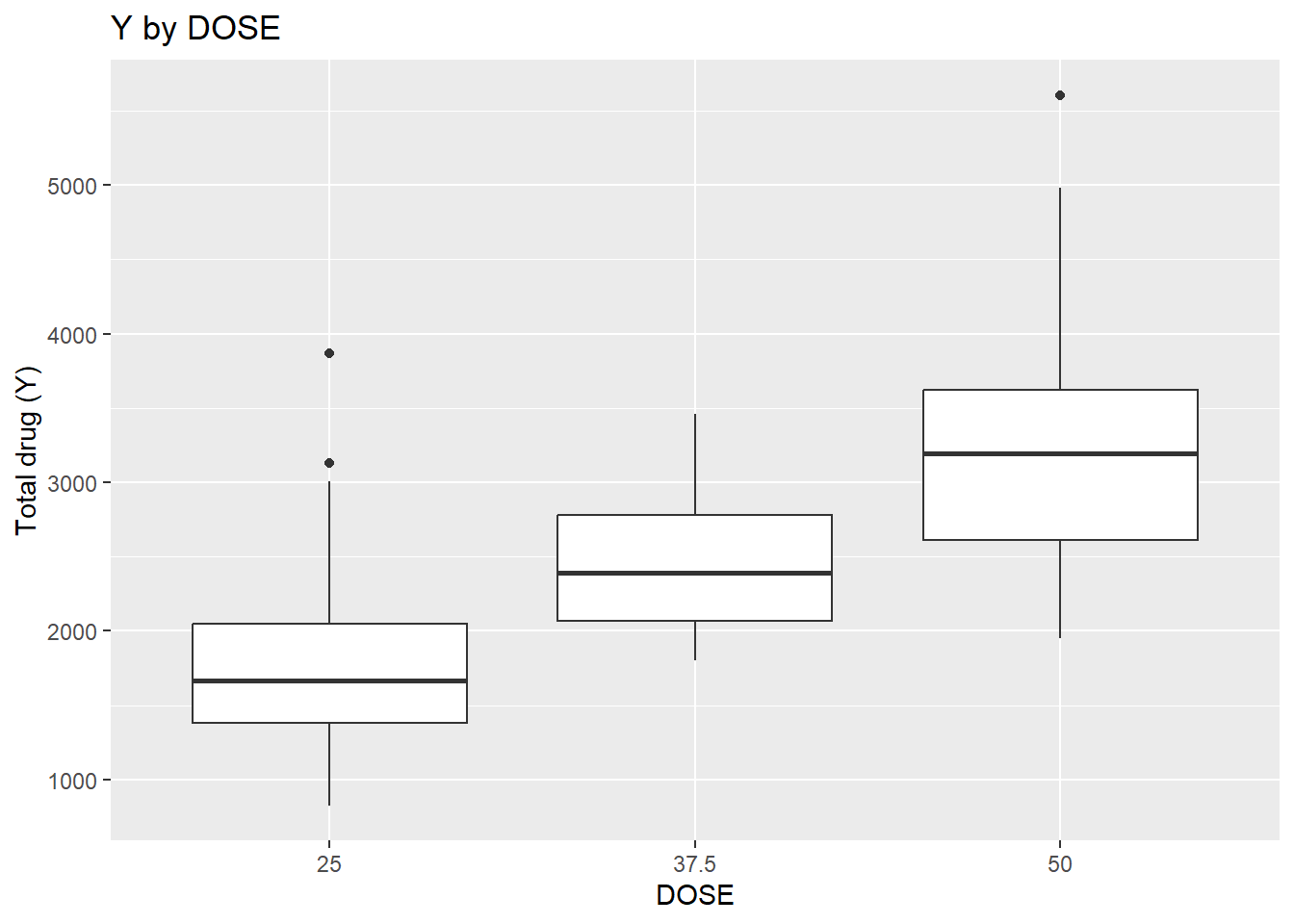
# Y vs DOSE 
ggplot(dat_clean, aes(x = factor(DOSE), y = Y)) +
  geom_boxplot() +
  labs(x = "DOSE", y = "Total drug (Y)", title = "Y by DOSE")

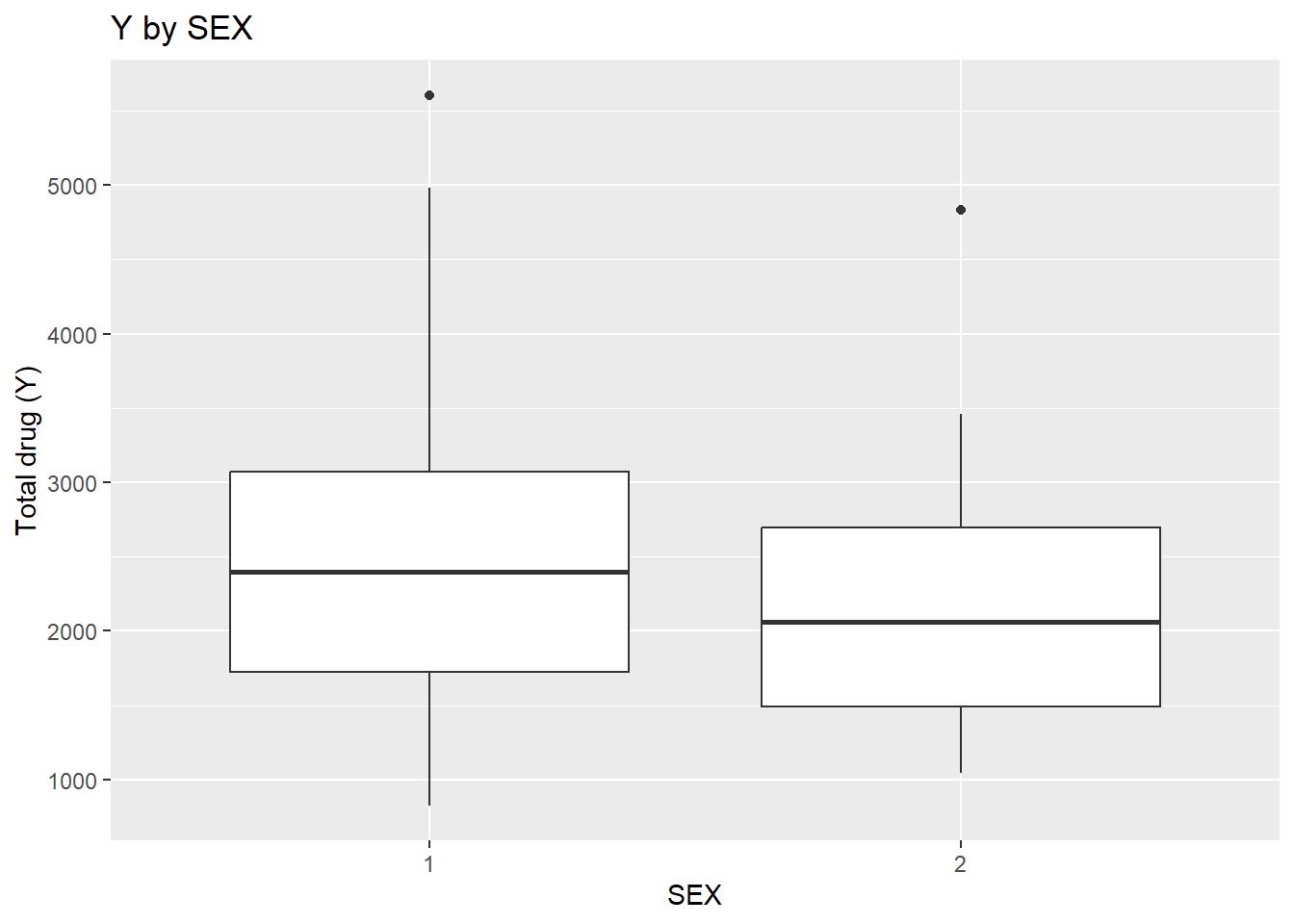
# Y vs SEX
ggplot(dat_clean, aes(x = SEX, y = Y)) +
  geom_boxplot() +
  labs(x = "SEX", y = "Total drug (Y)", title = "Y by SEX")

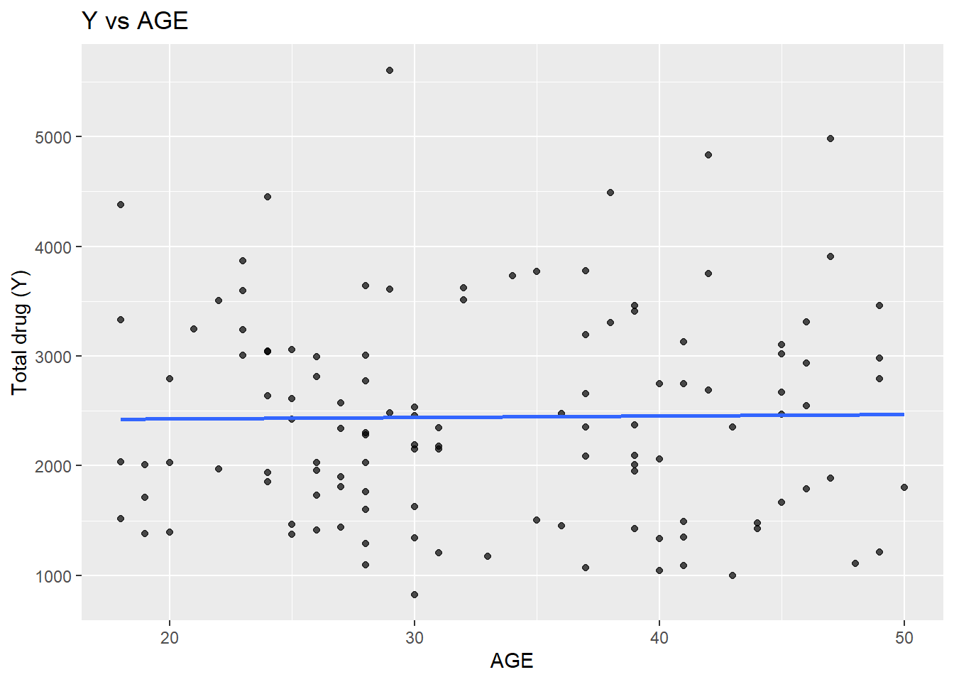
# Y vs AGE 
ggplot(dat_clean, aes(x = AGE, y = Y)) +
  geom_point(alpha = 0.7) +
  geom_smooth(method = "lm", se = FALSE) +
  labs(x = "AGE", y = "Total drug (Y)", title = "Y vs AGE")

`geom_smooth()` using formula = 'y ~ x'

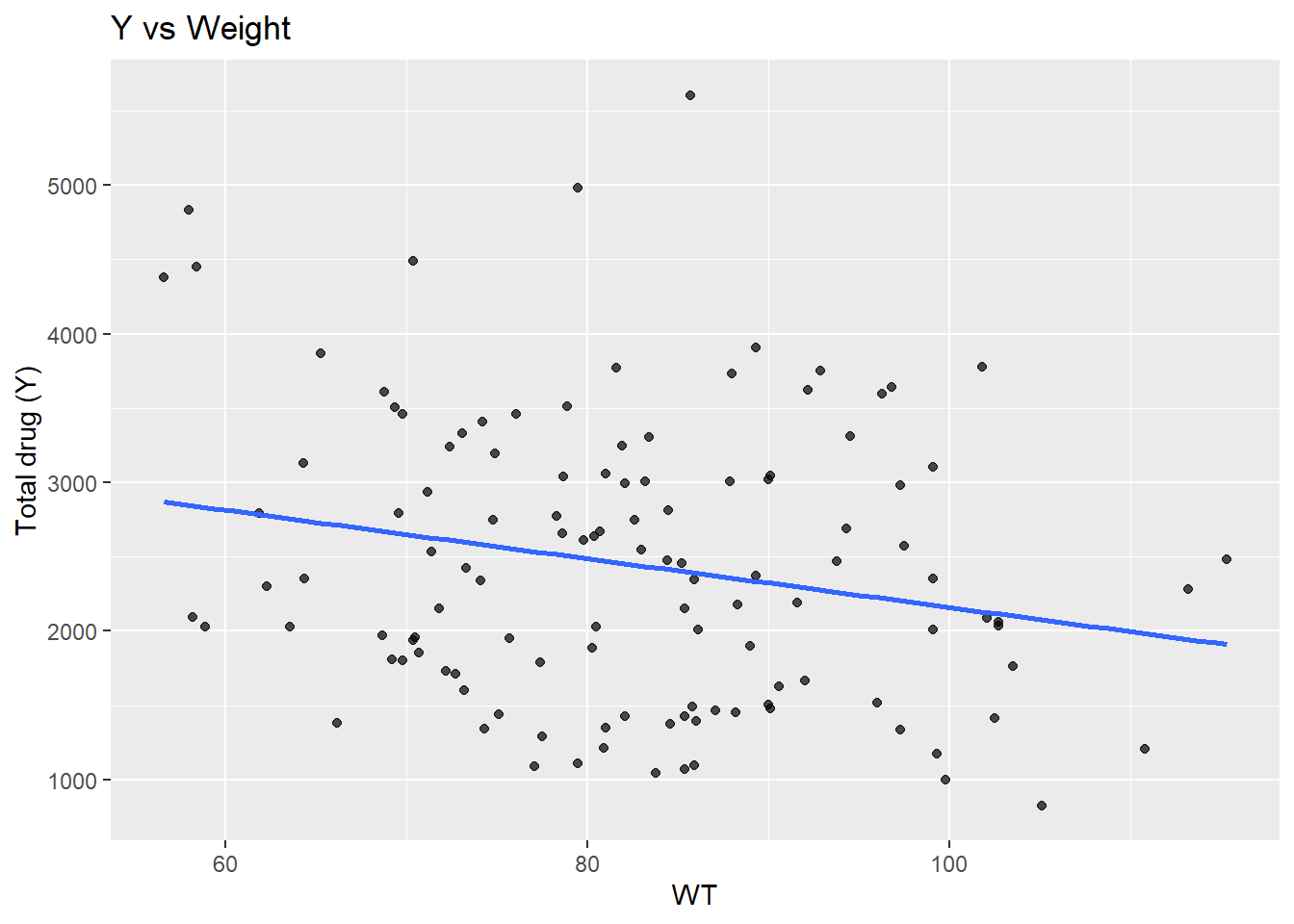
ggplot(dat_clean, aes(x = WT, y = Y)) +
  geom_point(alpha = 0.7) +
  geom_smooth(method = "lm", se = FALSE) +
  labs(x = "WT", y = "Total drug (Y)", title = "Y vs Weight")

`geom_smooth()` using formula = 'y ~ x'

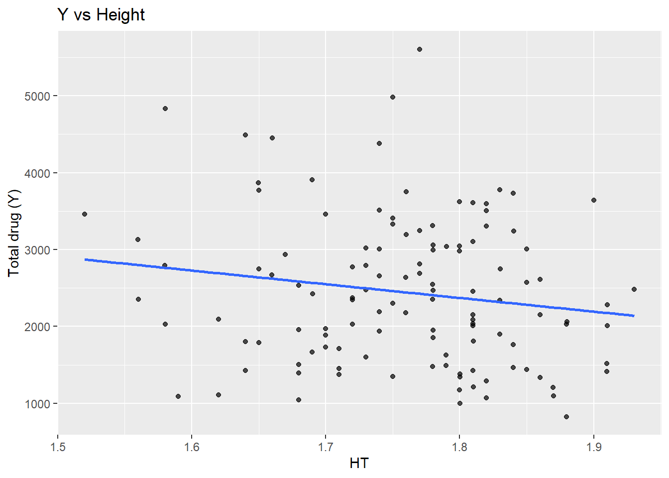
ggplot(dat_clean, aes(x = HT, y = Y)) +
  geom_point(alpha = 0.7) +
  geom_smooth(method = "lm", se = FALSE) +
  labs(x = "HT", y = "Total drug (Y)", title = "Y vs Height")

`geom_smooth()` using formula = 'y ~ x'

Distributions

dat_clean %>%
  pivot_longer(cols = c(Y, AGE, WT, HT),
               names_to = "variable", values_to = "value") %>%
  ggplot(aes(x = value)) +
  geom_histogram(bins = 30) +
  facet_wrap(~ variable, scales = "free") +
  labs(title = "Distributions of numeric variables")

Pair/correlation plots

# numeric-only correlation matrix
cor_mat <- dat_clean %>%
  select(Y, DOSE, AGE, WT, HT) %>%
  cor()

round(cor_mat, 2)

         Y DOSE   AGE    WT    HT
Y     1.00 0.72  0.01 -0.21 -0.16
DOSE  0.72 1.00  0.07  0.10  0.02
AGE   0.01 0.07  1.00  0.12 -0.35
WT   -0.21 0.10  0.12  1.00  0.60
HT   -0.16 0.02 -0.35  0.60  1.00

This suggests a strong positive relationship between Y and DOSE (cor ≈ 0.72), which is also visible in the boxplot of Y by dose. AGE shows little relationship with Y in this dataset. WT and HT are moderately correlated (cor ≈ 0.60).

Linear regression: Y - DOSE

library(tidymodels)

── Attaching packages ────────────────────────────────────── tidymodels 1.4.1 ──

✔ broom        1.0.12     ✔ rsample      1.3.2 
✔ dials        1.4.2      ✔ tailor       0.1.0 
✔ infer        1.1.0      ✔ tune         2.0.1 
✔ modeldata    1.5.1      ✔ workflows    1.3.0 
✔ parsnip      1.4.1      ✔ workflowsets 1.1.1 
✔ recipes      1.3.1      ✔ yardstick    1.3.2 

── Conflicts ───────────────────────────────────────── tidymodels_conflicts() ──
✖ scales::discard() masks purrr::discard()
✖ dplyr::filter()   masks stats::filter()
✖ recipes::fixed()  masks stringr::fixed()
✖ dplyr::lag()      masks stats::lag()
✖ yardstick::spec() masks readr::spec()
✖ recipes::step()   masks stats::step()

set.seed(123)

# split into training/testing
split1 <- initial_split(dat_clean, prop = 0.8)
train1 <- training(split1)
test1  <- testing(split1)

# model specification
lm_spec <- linear_reg() %>%
  set_engine("lm")

# workflow
wf_lm_dose <- workflow() %>%
  add_model(lm_spec) %>%
  add_formula(Y ~ DOSE)

# fit
fit_lm_dose <- fit(wf_lm_dose, data = train1)

# predict on test + metrics
pred_lm_dose <- predict(fit_lm_dose, new_data = test1) %>%
  bind_cols(test1 %>% select(Y))

metrics(pred_lm_dose, truth = Y, estimate = .pred) %>%
  filter(.metric %in% c("rmse", "rsq"))

# A tibble: 2 × 3
  .metric .estimator .estimate
  <chr>   <chr>          <dbl>
1 rmse    standard     483.   
2 rsq     standard       0.687

The linear model using DOSE as the only predictor explains approximately 69% of the variability in Y (R² ≈ 0.69). The RMSE is about 483 units, meaning that predictions are on average about 483 units away from the observed total drug value.

Linear regression: Y - all predictors

# workflow with all predictors
wf_lm_all <- workflow() %>%
  add_model(lm_spec) %>%
  add_formula(Y ~ DOSE + AGE + SEX + RACE + WT + HT)

# fit
fit_lm_all <- fit(wf_lm_all, data = train1)

# predict on test + metrics
pred_lm_all <- predict(fit_lm_all, new_data = test1) %>%
  bind_cols(test1 %>% select(Y))

metrics(pred_lm_all, truth = Y, estimate = .pred) %>%
  filter(.metric %in% c("rmse", "rsq"))

# A tibble: 2 × 3
  .metric .estimator .estimate
  <chr>   <chr>          <dbl>
1 rmse    standard     494.   
2 rsq     standard       0.662

Adding AGE, SEX, RACE, WT, and HT did not improve predictive performance. In fact, the test-set RMSE increased slightly (483 to 494) and R² decreased (0.687 to 0.662). This suggests that DOSE already captures most of the explainable variation in Y, and the additional predictors add little signal (or add noise) in this dataset.

Logistic regression: SEX - DOSE

set.seed(123)

split2 <- initial_split(dat_clean, prop = 0.8, strata = SEX)
train2 <- training(split2)
test2  <- testing(split2)

# logistic model specification
log_spec <- logistic_reg() %>%
  set_engine("glm")


wf_log_dose <- workflow() %>%
  add_model(log_spec) %>%
  add_formula(SEX ~ DOSE)

# fit
fit_log_dose <- fit(wf_log_dose, data = train2)

# predict probabilities
pred_log_dose <- predict(fit_log_dose, test2, type = "prob") %>%
  bind_cols(predict(fit_log_dose, test2)) %>%
  bind_cols(test2 %>% select(SEX))

# compute metrics
metric_set(accuracy, roc_auc)(pred_log_dose,
                              truth = SEX,
                              estimate = .pred_class,
                              .pred_1)

# A tibble: 2 × 3
  .metric  .estimator .estimate
  <chr>    <chr>          <dbl>
1 accuracy binary         0.84 
2 roc_auc  binary         0.494

The model shows high accuracy (0.84), but the ROC-AUC is ~0.49, which is essentially random (≈0.5). The high accuracy is likely driven by class imbalance (most observations are in one SEX category), so a model that predicts the majority class most of the time can achieve high accuracy without being truly predictive. Overall, DOSE does not appear to meaningfully predict SEX.

Logistic regression: SEX - all predictors

set.seed(123)

# split
split2 <- initial_split(dat_clean, prop = 0.8, strata = SEX)
train2 <- training(split2)
test2  <- testing(split2)

# logistic model specification
log_spec <- logistic_reg() %>%
  set_engine("glm")

# with all predictors
wf_log_all <- workflow() %>%
  add_model(log_spec) %>%
  add_formula(SEX ~ DOSE + AGE + RACE + WT + HT)

# fit
fit_log_all <- fit(wf_log_all, data = train2)

# predict probabilities + classes on test set
pred_log_all <- predict(fit_log_all, test2, type = "prob") %>%
  bind_cols(predict(fit_log_all, test2)) %>%   # adds .pred_class
  bind_cols(test2 %>% select(SEX))

# compute metrics
metric_set(accuracy, roc_auc)(
  pred_log_all,
  truth = SEX,
  estimate = .pred_class,
  .pred_1
)

# A tibble: 2 × 3
  .metric  .estimator .estimate
  <chr>    <chr>          <dbl>
1 accuracy binary             1
2 roc_auc  binary             1

The model achieved very high performance on this test split, but the test set is small and imbalanced, so these metrics may be unstable or overly optimistic. Results should be interpreted carefully.

Summary

Overall, DOSE was a strong predictor of the continuous outcome Y, explaining a substantial portion of its variability. Adding additional baseline predictors did not improve performance meaningfully. For the categorical outcome SEX, predictive performance varied depending on the model and evaluation strategy, and results should be interpreted carefully due to class imbalance. This exercise illustrates the complete modeling workflow, including data splitting, model fitting, prediction, and evaluation.

Module 10: Model Improvement

Data Prep

# remove RACE variable
data6 <- dat_person %>%
  mutate(
    SEX = factor(SEX)
  ) %>%
  select(Y, DOSE, AGE, SEX, WT, HT) %>%
  mutate(
    SEX = forcats::fct_drop(SEX)
  )

# set seed
rngseed <- 1234
set.seed(rngseed)

# data split
data_split <- initial_split(data6, prop = 3/4)

# create train/test sets
train_data <- training(data_split)
test_data  <- testing(data_split)

Model Fitting

library(tidymodels)

# model specification
lm_mod <- linear_reg() %>%
  set_engine("lm")

# fit model 1 (Y ~ DOSE)
lm_fit_10_1 <- lm_mod %>%
  fit(Y ~ DOSE, data = train_data)

lm_fit_10_1

parsnip model object


Call:
stats::lm(formula = Y ~ DOSE, data = data)

Coefficients:
(Intercept)         DOSE  
     535.45        53.42  

# fit model 2 (Y ~ all predictors)
lm_fit_10_2 <- lm_mod %>%
  fit(Y ~ ., data = train_data)

lm_fit_10_2

parsnip model object


Call:
stats::lm(formula = Y ~ ., data = data)

Coefficients:
(Intercept)         DOSE          AGE         SEX2           WT           HT  
  4396.7716      55.3445      -0.4174    -568.9967     -22.6399   -1129.6696  

Model Performance Assessment 1

# predictions for model 1
preds_10_1 <- predict(lm_fit_10_1, new_data = train_data) %>%
  bind_cols(train_data %>% select(Y))

rmse(preds_10_1, truth = Y, estimate = .pred)

# A tibble: 1 × 3
  .metric .estimator .estimate
  <chr>   <chr>          <dbl>
1 rmse    standard        703.

rsq(preds_10_1, truth = Y, estimate = .pred)

# A tibble: 1 × 3
  .metric .estimator .estimate
  <chr>   <chr>          <dbl>
1 rsq     standard       0.451

# predictions for model 2
preds_10_2 <- predict(lm_fit_10_2, new_data = train_data) %>%
  bind_cols(train_data %>% select(Y))

rmse(preds_10_2, truth = Y, estimate = .pred)

# A tibble: 1 × 3
  .metric .estimator .estimate
  <chr>   <chr>          <dbl>
1 rmse    standard        627.

rsq(preds_10_2, truth = Y, estimate = .pred)

# A tibble: 1 × 3
  .metric .estimator .estimate
  <chr>   <chr>          <dbl>
1 rsq     standard       0.562

# null model
null_mod <- null_model(mode = "regression") %>%
  set_engine("parsnip")

null_fit <- null_mod %>%
  fit(Y ~ 1, data = train_data)

null_preds <- predict(null_fit, new_data = train_data) %>%
  bind_cols(train_data %>% select(Y))

rmse(null_preds, truth = Y, estimate = .pred)

# A tibble: 1 × 3
  .metric .estimator .estimate
  <chr>   <chr>          <dbl>
1 rmse    standard        948.

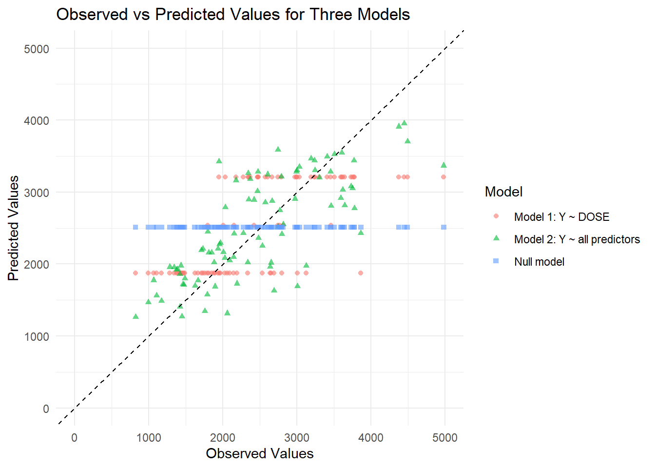
The null model shows the highest RMSE, indicating the poorest performance. The DOSE-only model performs better, while the model including all predictors achieves the lowest RMSE. This suggests that adding AGE, SEX, WT, and HT improves prediction of Y compared to using DOSE alone.

Model Performance Assessment 2

# create 10-fold cross-validation splits
set.seed(rngseed)
folds <- vfold_cv(train_data, v = 10)

# perform cross-validation for model 1
cv_fit1 <- lm_mod %>%
  fit_resamples(
    Y ~ DOSE,
    resamples = folds,
    metrics = metric_set(rmse)
  )

collect_metrics(cv_fit1)

# A tibble: 1 × 6
  .metric .estimator  mean     n std_err .config        
  <chr>   <chr>      <dbl> <int>   <dbl> <chr>          
1 rmse    standard    691.    10    67.5 pre0_mod0_post0

# perform cross-validation for model 2
cv_fit2 <- lm_mod %>%
  fit_resamples(
    Y ~ .,
    resamples = folds,
    metrics = metric_set(rmse)
  )

collect_metrics(cv_fit2)

# A tibble: 1 × 6
  .metric .estimator  mean     n std_err .config        
  <chr>   <chr>      <dbl> <int>   <dbl> <chr>          
1 rmse    standard    646.    10    64.8 pre0_mod0_post0

Using 10-fold cross-validation, the RMSE for the DOSE-only model was approximately 691, while the model including all predictors achieved a lower RMSE of about 646. Compared to the earlier training-based estimates, the RMSE values are slightly higher, which is expected since cross-validation provides a more realistic estimate of performance on unseen data.

The model with all predictors still performs better than the DOSE-only model, indicating that the additional variables provide some predictive value when evaluated more robustly. The standard errors indicate some variability across folds, reflecting the limited sample size and the impact of random data splitting.

# run CV again with a different seed
rngseed2 <- 5678
set.seed(rngseed2)

folds2 <- vfold_cv(train_data, v = 10)

cv_fit3 <- lm_mod %>%
  fit_resamples(
    Y ~ DOSE,
    resamples = folds2,
    metrics = metric_set(rmse)
  )

collect_metrics(cv_fit3)

# A tibble: 1 × 6
  .metric .estimator  mean     n std_err .config        
  <chr>   <chr>      <dbl> <int>   <dbl> <chr>          
1 rmse    standard    693.    10    62.8 pre0_mod0_post0

cv_fit4 <- lm_mod %>%
  fit_resamples(
    Y ~ .,
    resamples = folds2,
    metrics = metric_set(rmse)
  )

collect_metrics(cv_fit4)

# A tibble: 1 × 6
  .metric .estimator  mean     n std_err .config        
  <chr>   <chr>      <dbl> <int>   <dbl> <chr>          
1 rmse    standard    649.    10    54.4 pre0_mod0_post0

Repeating the cross-validation with a different random seed resulted in slightly different RMSE values for both models. This variation is expected due to randomness in the data splitting process. However, the overall pattern remained consistent, with the model including all predictors continuing to outperform the DOSE-only model.

This section is added by Austin Hill

# load packages 
library(tidyverse)
library(tidymodels)

# Create a combined data frame of observed and predicted values for all 3 original models

# Model 1 plotting data
model1_plot_df <- preds_10_1 %>%
  rename(observed = Y) %>%
  mutate(model = "Model 1: Y ~ DOSE")

# Model 2 plotting data
model2_plot_df <- preds_10_2 %>%
  rename(observed = Y) %>%
  mutate(model = "Model 2: Y ~ all predictors")

# Null model plotting data
null_plot_df <- null_preds %>%
  rename(observed = Y) %>%
  mutate(model = "Null model")

# Combine all three models into one data frame
all_model_preds <- bind_rows(
  model1_plot_df,
  model2_plot_df,
  null_plot_df
)

# Inspect combined plotting data
glimpse(all_model_preds)

Rows: 270
Columns: 3
$ .pred    <dbl> 3206.650, 1871.052, 2538.851, 1871.052, 3206.650, 1871.052, 1…
$ observed <dbl> 3004.21, 1346.62, 2771.69, 2027.60, 2353.40, 826.43, 3865.79,…
$ model    <chr> "Model 1: Y ~ DOSE", "Model 1: Y ~ DOSE", "Model 1: Y ~ DOSE"…

# Plot observed vs predicted for all 3 models

ggplot(
  all_model_preds,
  aes(x = observed, y = .pred, color = model, shape = model)
) +
  geom_point(alpha = 0.6) +
  geom_abline(slope = 1, intercept = 0, linetype = "dashed") +
  coord_cartesian(xlim = c(0, 5000), ylim = c(0, 5000)) +
  labs(
    title = "Observed vs Predicted Values for Three Models",
    x = "Observed Values",
    y = "Predicted Values",
    color = "Model",
    shape = "Model"
  ) +
  theme_minimal()

# Create residuals for Model 2

model2_resid_df <- preds_10_2 %>%
  rename(observed = Y) %>%
  mutate(residual = .pred - observed) %>%
  select(observed, .pred, residual)

glimpse(model2_resid_df)

Rows: 90
Columns: 3
$ observed <dbl> 3004.21, 1346.62, 2771.69, 2027.60, 2353.40, 826.43, 3865.79,…
$ .pred    <dbl> 3303.028, 1952.556, 2744.878, 2081.182, 2894.205, 1264.763, 2…
$ residual <dbl> 298.81777, 605.93586, -26.81172, 53.58237, 540.80500, 438.333…

# Create symmetric y-axis limits

max_abs_resid <- max(abs(model2_resid_df$residual), na.rm = TRUE)

# Plot predicted vs residuals for Model 2

ggplot(model2_resid_df, aes(x = .pred, y = residual)) +
  geom_point(alpha = 0.6) +
  geom_hline(yintercept = 0, linetype = "dashed") +
  coord_cartesian(ylim = c(-max_abs_resid, max_abs_resid)) +
  labs(
    title = "Predicted Values vs Residuals for Model 2",
    x = "Predicted Values",
    y = "Residuals (Predicted - Observed)"
  ) +
  theme_minimal()

# Re-set seed and create 100 bootstrap samples using the training data

set.seed(rngseed)

boot_splits <- bootstraps(train_data, times = 100)

boot_splits

# Bootstrap sampling 
# A tibble: 100 × 2
   splits          id          
   <list>          <chr>       
 1 <split [90/33]> Bootstrap001
 2 <split [90/32]> Bootstrap002
 3 <split [90/26]> Bootstrap003
 4 <split [90/39]> Bootstrap004
 5 <split [90/32]> Bootstrap005
 6 <split [90/38]> Bootstrap006
 7 <split [90/36]> Bootstrap007
 8 <split [90/38]> Bootstrap008
 9 <split [90/32]> Bootstrap009
10 <split [90/33]> Bootstrap010
# ℹ 90 more rows

# Fit Model 2 to each bootstrap sample and predict on the original training data

boot_pred_list <- map(boot_splits$splits, function(split) {
  
  boot_train <- analysis(split)
  
  # Re-fit Model 2 using the same model spec as before
  boot_fit <- lm_mod %>%
    fit(Y ~ ., data = boot_train)
  
  # Predict on the original training data
  predict(boot_fit, new_data = train_data) %>%
    pull(.pred)
})

# Convert bootstrap predictions to a matrix
# Rows = training observations
# Columns = bootstrap samples

boot_pred_mat <- do.call(cbind, boot_pred_list)

dim(boot_pred_mat)

[1]  90 100

# Create summary data frame with observed values, original point estimates, and bootstrap summaries

boot_summary_df <- tibble(
  observed = train_data$Y,
  point_estimate = preds_10_2$.pred,
  boot_mean = apply(boot_pred_mat, 1, mean, na.rm = TRUE),
  boot_median = apply(boot_pred_mat, 1, median, na.rm = TRUE),
  lower_ci = apply(boot_pred_mat, 1, quantile, probs = 0.025, na.rm = TRUE),
  upper_ci = apply(boot_pred_mat, 1, quantile, probs = 0.975, na.rm = TRUE)
)

glimpse(boot_summary_df)

Rows: 90
Columns: 6
$ observed       <dbl> 3004.21, 1346.62, 2771.69, 2027.60, 2353.40, 826.43, 38…
$ point_estimate <dbl> 3303.028, 1952.556, 2744.878, 2081.182, 2894.205, 1264.…
$ boot_mean      <dbl> 3327.341, 1944.126, 2757.878, 2073.550, 2914.454, 1283.…
$ boot_median    <dbl> 3335.818, 1945.359, 2764.634, 2085.856, 2933.091, 1298.…
$ lower_ci       <dbl> 3083.086, 1645.772, 2556.181, 1722.745, 2645.607, 1001.…
$ upper_ci       <dbl> 3586.619, 2232.636, 2974.479, 2435.738, 3197.893, 1547.…

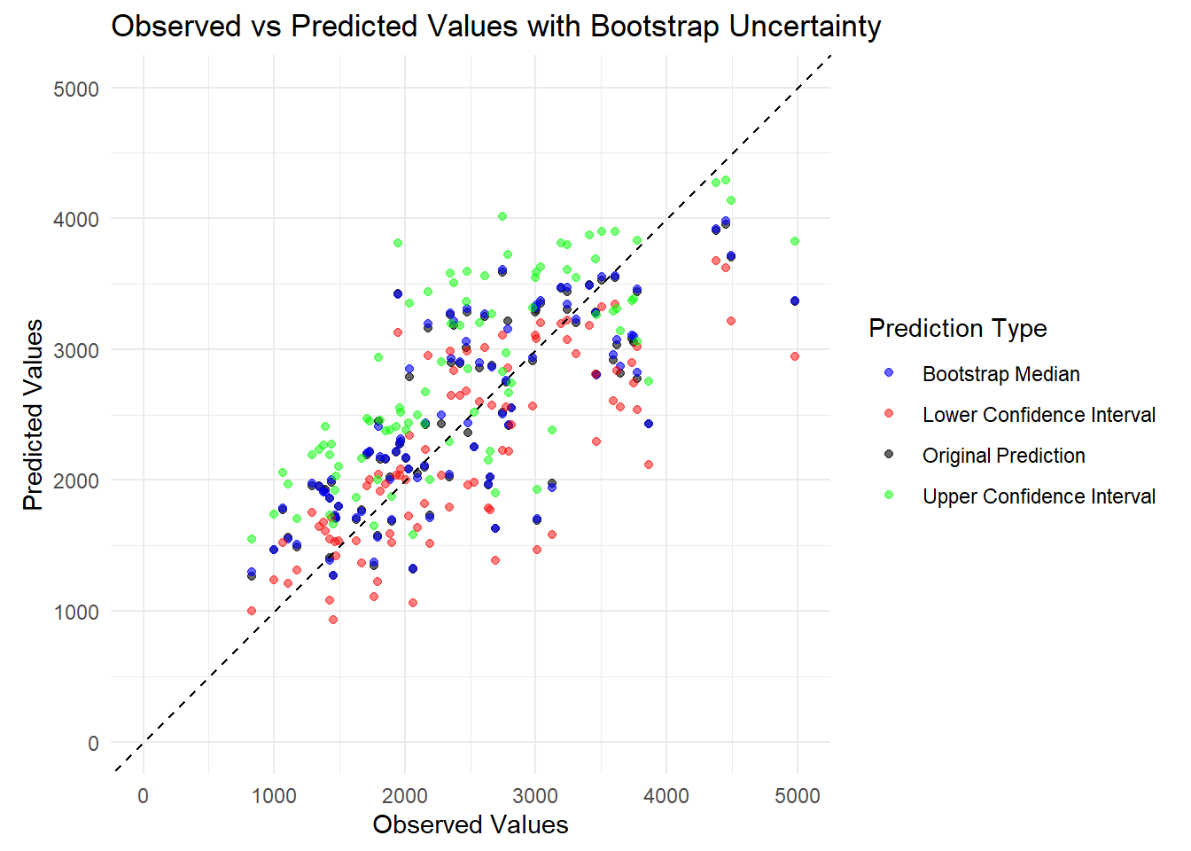
# Plot observed values vs original predictions,bootstrap median, and bootstrap CI limits

ggplot(boot_summary_df, aes(x = observed)) +
  geom_point(aes(y = point_estimate, color = "Original Prediction"), alpha = 0.6) +
  geom_point(aes(y = boot_median, color = "Bootstrap Median"), alpha = 0.6) +
  geom_point(aes(y = lower_ci, color = "Lower Confidence Interval"), alpha = 0.5) +
  geom_point(aes(y = upper_ci, color = "Upper Confidence Interval"), alpha = 0.5) +
  
  geom_abline(slope = 1, intercept = 0, linetype = "dashed") +
  
  scale_color_manual(
    name = "Prediction Type",
    values = c(
      "Original Prediction" = "black", 
      "Bootstrap Median" = "blue", 
      "Lower Confidence Interval" = "red", # Added missing comma here
      "Upper Confidence Interval" = "green" # Fixed capitalization to match above
    )
  ) +
  
  coord_equal(xlim = c(0, 5000), ylim = c(0, 5000)) +
  labs(
    title = "Observed vs Predicted Values with Bootstrap Uncertainty",
    x = "Observed Values",
    y = "Predicted Values"
  ) +
  theme_minimal()

Discussion

This plot shows that the model is moderately accurate, as the points generally cluster around the dashed 45-degree line, though there is a noticeable amount of scatter. The vertical distance between the green (upper) and red (lower) points reveals maybe some prediction uncertainty. The black and blue dots are very tightly clustered. This means the model’s central tendency is reliable and isn’t being wildly tossed around by small changes in the training data.

# final evaluation on test data

# predictions for model 2 on training data
pred_train_m2 <- predict(lm_fit_10_2, new_data = train_data) %>%
  bind_cols(train_data %>% select(Y)) %>%
  mutate(dataset = "Train")

# predictions for model 2 on test data
pred_test_m2 <- predict(lm_fit_10_2, new_data = test_data) %>%
  bind_cols(test_data %>% select(Y)) %>%
  mutate(dataset = "Test")

head(pred_train_m2)

# A tibble: 6 × 3
  .pred     Y dataset
  <dbl> <dbl> <chr>  
1 3303. 3004. Train  
2 1953. 1347. Train  
3 2745. 2772. Train  
4 2081. 2028. Train  
5 2894. 2353. Train  
6 1265.  826. Train  

head(pred_test_m2)

# A tibble: 6 × 3
  .pred     Y dataset
  <dbl> <dbl> <chr>  
1 1871. 2549. Test   
2 2665. 2353. Test   
3 2357. 2009. Test   
4 2954. 2934. Test   
5 2101. 2085. Test   
6 3479. 4835. Test   

pred_both_m2 <- bind_rows(pred_train_m2, pred_test_m2)

head(pred_both_m2)

# A tibble: 6 × 3
  .pred     Y dataset
  <dbl> <dbl> <chr>  
1 3303. 3004. Train  
2 1953. 1347. Train  
3 2745. 2772. Train  
4 2081. 2028. Train  
5 2894. 2353. Train  
6 1265.  826. Train  

table(pred_both_m2$dataset)

 Test Train 
   30    90 

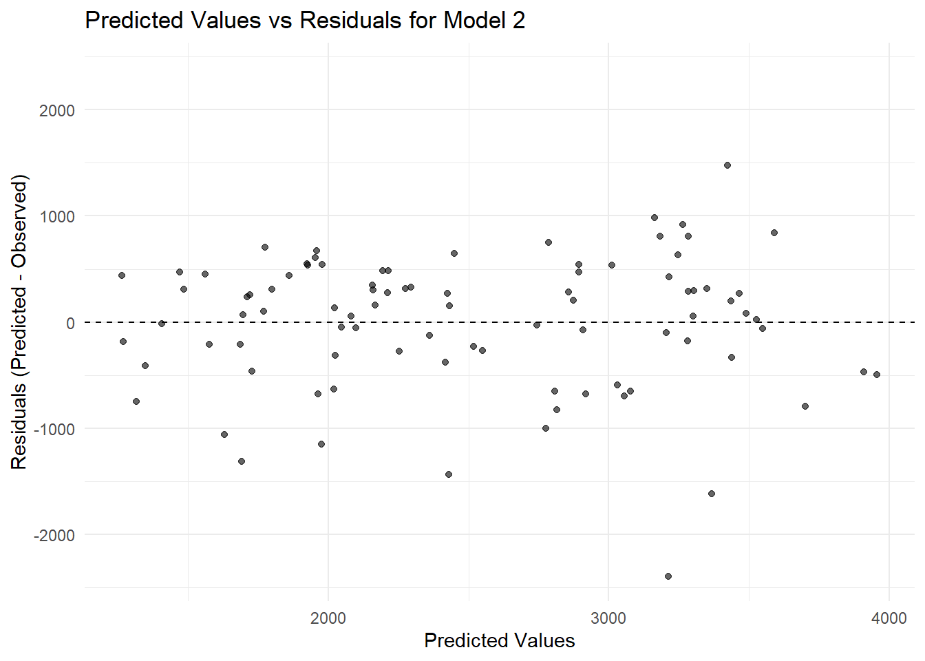
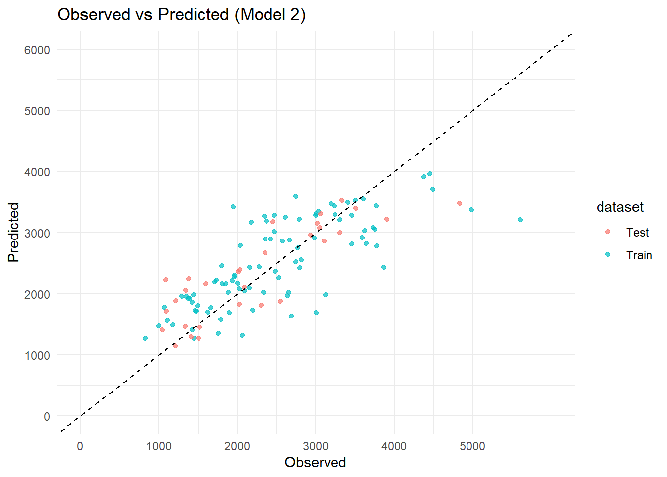
library(ggplot2)

ggplot(pred_both_m2, aes(x = Y, y = .pred, color = dataset)) +
  geom_point(alpha = 0.7) +
  geom_abline(slope = 1, intercept = 0, linetype = "dashed") +
  scale_x_continuous(limits = c(0, 6000), breaks = seq(0, 5500, by = 1000)) +
  scale_y_continuous(limits = c(0, 6000), breaks = seq(0, 6000, by = 1000)) +
  labs(
    title = "Observed vs Predicted (Model 2)",
    x = "Observed",
    y = "Predicted"
  ) +
  theme_minimal()

Final evaluation using the test data showed that predictions from model 2 generalize well to unseen data. In the combined plot, the test data points are mixed with the training data and follow a similar trend along the diagonal line, indicating that the model is not overfitting and performs consistently across both datasets.

library(yardstick)

# RMSE for training
rmse_train <- rmse(pred_train_m2, truth = Y, estimate = .pred)

# RMSE for test
rmse_test <- rmse(pred_test_m2, truth = Y, estimate = .pred)

rmse_train

# A tibble: 1 × 3
  .metric .estimator .estimate
  <chr>   <chr>          <dbl>
1 rmse    standard        627.

rmse_test

# A tibble: 1 × 3
  .metric .estimator .estimate
  <chr>   <chr>          <dbl>
1 rmse    standard        520.

The RMSE values for the training and test datasets are close, indicating that the model performs consistently on both datasets. The slightly lower RMSE for the test data suggests that the model generalizes well and does not show evidence of overfitting.

Overall model assessment

To assess the models, I compared their RMSE values on the training data, their cross-validation performance, and the final test-set behavior of model 2. Lower RMSE indicates better predictive performance. Both model 1 and model 2 performed better than the null model, indicating that including predictors improves prediction accuracy. Model 1 has lower RMSE compared with the null model, indicating that DOSE is an important predictor of Y and has a meaningful relationship with the outcome. Model 2 further improved performance beyond model 1. This suggests that adding AGE, SEX, WT, and HT provided additional predictive information beyond DOSE alone. The cross-validation results supported the same pattern, with model 2 continuing to have a lower RMSE than model 1, which makes the improvement more convincing and less likely to be due only to the particular training set split. The final test-set evaluation of model 2 also suggested that the model generalizes reasonably well. The test points were mixed with the training points in the observed versus predicted plot, and the training and test RMSE values were closer. Overall, model 1 is useful as a simple baseline model, but it is probably too limited for more reliable prediction on its own. Model 2 is the strongest model among those considered here and appears more useful because it performs better and generalizes reasonably well, although it is still not a perfect predictor since there is still noticeable spread around the diagonal in the prediction plot.