Data Exercise – Synthetic Data

This synthetic data example was inspired by the synthetic data demonstrations provided in MADA course Model4.

Introduction

For this example, we generate a simple dataset for a hypothetical dietary intervention and its impact on outcomes such as body weight and gastrointestinal side effects. The data are fully synthetic and are used to demonstrate data generation, exploration, and simple modeling.

Data generation

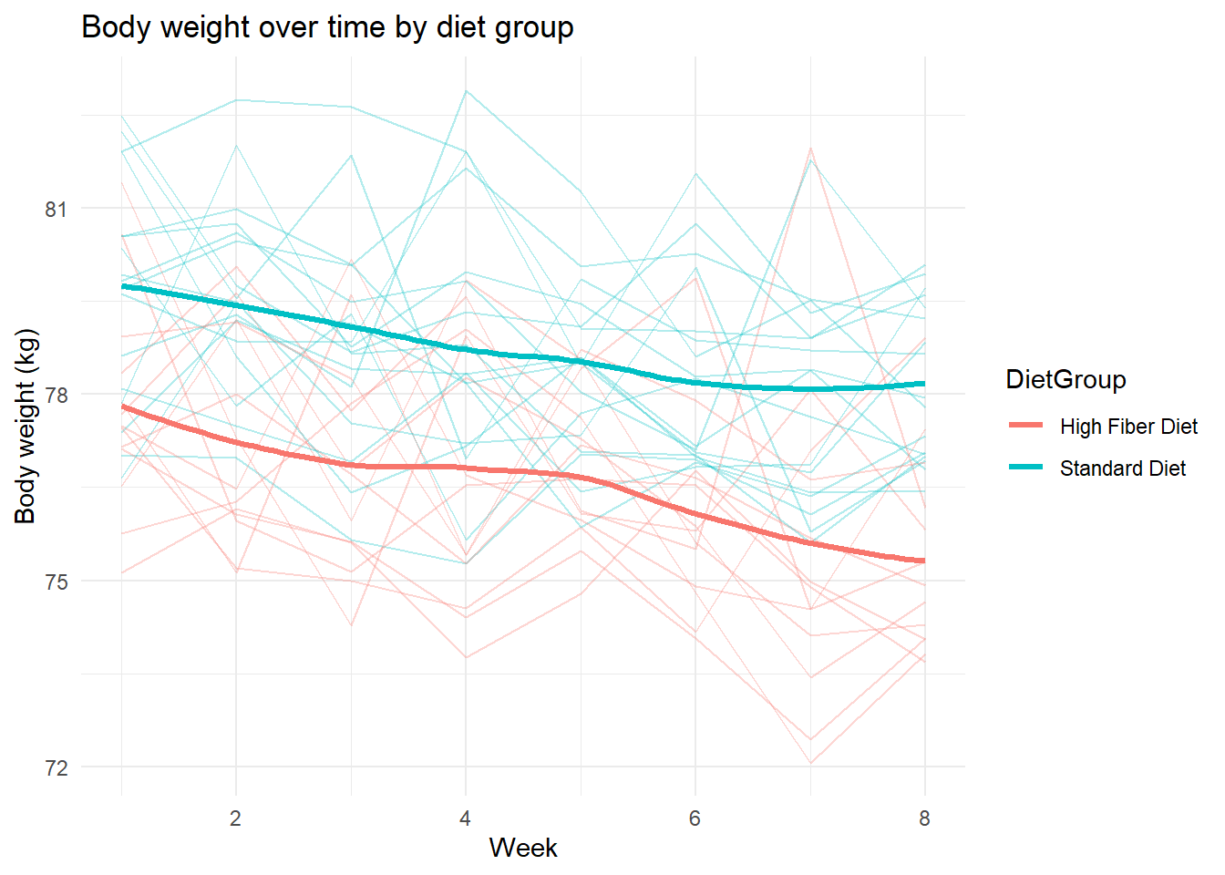
We generate synthetic data for a hypothetical dietary intervention study. Individuals are assigned to one of two diet groups and followed over time. Body weight and gastrointestinal side effects are recorded.

# Set seed for reproducibility
set.seed(123)

# Number of participants
n_participants <- 30

# Number of weeks
n_weeks <- 8

# Diet groups
diet_groups <- c("Standard Diet", "High Fiber Diet")

# Participant-level data
participants <- data.frame(
  ParticipantID = 1:n_participants,
  DietGroup = sample(diet_groups, n_participants, replace = TRUE),
  Age = round(rnorm(n_participants, mean = 40, sd = 12))
)

# Expand to weekly observations
diet_data <- participants[rep(1:n_participants, each = n_weeks), ]
diet_data$Week <- rep(1:n_weeks, times = n_participants)

# Generate body weight (kg)
diet_data$BodyWeight <- with(diet_data, {
  baseline <- ifelse(DietGroup == "Standard Diet", 80, 78)
  age_effect <- 0.08 * (Age - 40)
  week_effect <- -0.3 * Week
  noise <- rnorm(nrow(diet_data), mean = 0, sd = 1.5)

  baseline + age_effect + week_effect + noise
})

# Probability of gastrointestinal side effects
gi_prob <- plogis((diet_data$BodyWeight - 75) / 5)

diet_data$GISideEffect <- rbinom(
  nrow(diet_data),
  size = 1,
  prob = gi_prob
)

# Check data
head(diet_data)

    ParticipantID     DietGroup Age Week BodyWeight GISideEffect
1               1 Standard Diet  61    1   79.69534            1
1.1             1 Standard Diet  61    2   80.47567            0
1.2             1 Standard Diet  61    3   80.08002            1
1.3             1 Standard Diet  61    4   81.64995            1
1.4             1 Standard Diet  61    5   80.05495            0
1.5             1 Standard Diet  61    6   80.25998            1

table(diet_data$DietGroup)

High Fiber Diet   Standard Diet 
            104             136 

summary(diet_data$Age)

   Min. 1st Qu.  Median    Mean 3rd Qu.    Max. 
   16.0    32.0    38.5    40.2    50.0    66.0 

Data exploration

Now exploring the structure of the synthetic dataset and summarizing key variables to confirm that the data were generated as expected.

# Check the size of the dataset
dim(diet_data)

[1] 240   6

# Check variable types and structure
str(diet_data)

'data.frame':   240 obs. of  6 variables:
 $ ParticipantID: int  1 1 1 1 1 1 1 1 2 2 ...
 $ DietGroup    : chr  "Standard Diet" "Standard Diet" "Standard Diet" "Standard Diet" ...
 $ Age          : num  61 61 61 61 61 61 61 61 46 46 ...
 $ Week         : int  1 2 3 4 5 6 7 8 1 2 ...
 $ BodyWeight   : num  79.7 80.5 80.1 81.6 80.1 ...
 $ GISideEffect : int  1 0 1 1 0 1 1 1 1 1 ...

# Summary of body weight
summary(diet_data$BodyWeight)

   Min. 1st Qu.  Median    Mean 3rd Qu.    Max. 
  72.07   76.34   77.76   77.79   79.30   82.90 

# Check diet group distribution
table(diet_data$DietGroup)

High Fiber Diet   Standard Diet 
            104             136 

Data visualization

We visualize trends in body weight over time and compare outcomes between diet groups to explore patterns in the synthetic data.

library(ggplot2)

ggplot(diet_data, aes(x = Week, y = BodyWeight, color = DietGroup)) +
  geom_line(aes(group = ParticipantID), alpha = 0.3) +
  geom_smooth(se = FALSE, linewidth = 1.2) +
  labs(
    title = "Body weight over time by diet group",
    x = "Week",
    y = "Body weight (kg)"
  ) +
  theme_minimal()

`geom_smooth()` using method = 'loess' and formula = 'y ~ x'

ggplot(diet_data, aes(x = Age, y = BodyWeight)) +
  geom_point(alpha = 0.6) +
  labs(
    title = "Body weight vs age",
    x = "Age (years)",
    y = "Body weight (kg)"
  ) +
  theme_minimal()

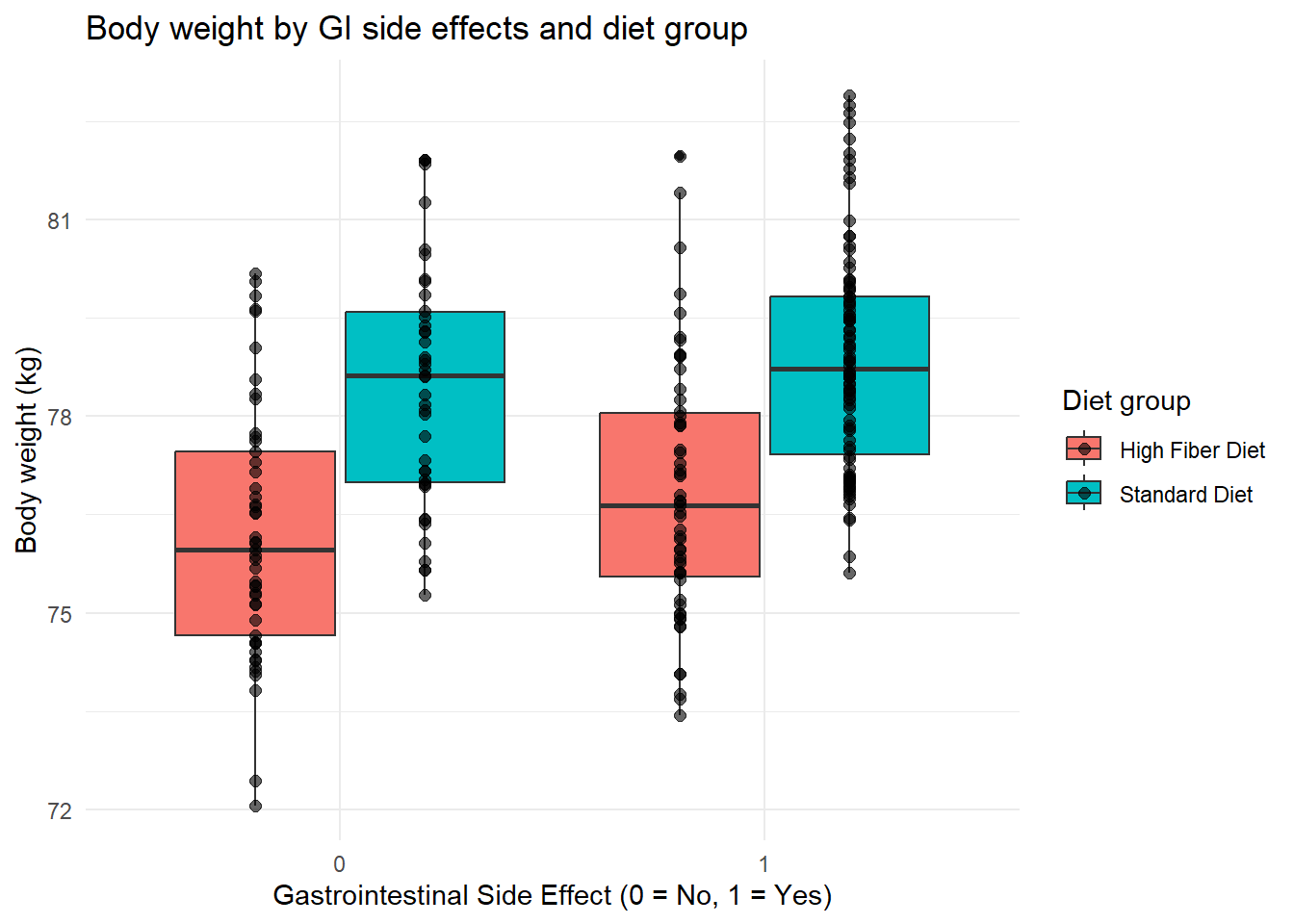
ggplot(diet_data,
       aes(x = as.factor(GISideEffect),
           y = BodyWeight,
           fill = DietGroup)) +
  geom_boxplot(position = position_dodge(width = 0.8)) +
  geom_point(position = position_dodge(width = 0.8),
             alpha = 0.6, size = 2) +
  labs(
    x = "Gastrointestinal Side Effect (0 = No, 1 = Yes)",
    y = "Body weight (kg)",
    title = "Body weight by GI side effects and diet group",
    fill = "Diet group"
  ) +
  theme_minimal()

Simple modeling

We fit simple models to assess the association between diet group, time, and body weight, as well as the relationship between body weight and the probability of gastrointestinal side effects.

# Linear model: body weight as a function of time, diet group, and age
model_weight <- lm(
  BodyWeight ~ Week + DietGroup + Age,
  data = diet_data
)
summary(model_weight)

Call:
lm(formula = BodyWeight ~ Week + DietGroup + Age, data = diet_data)

Residuals:
    Min      1Q  Median      3Q     Max 
-3.4388 -0.8793 -0.1217  0.8367  4.8225 

Coefficients:
                        Estimate Std. Error t value Pr(>|t|)    
(Intercept)            74.621824   0.376468 198.215  < 2e-16 ***
Week                   -0.288293   0.039857  -7.233 6.55e-12 ***
DietGroupStandard Diet  2.032900   0.185015  10.988  < 2e-16 ***
Age                     0.082460   0.007706  10.701  < 2e-16 ***
---
Signif. codes:  0 '***' 0.001 '**' 0.01 '*' 0.05 '.' 0.1 ' ' 1

Residual standard error: 1.415 on 236 degrees of freedom
Multiple R-squared:  0.568, Adjusted R-squared:  0.5625 
F-statistic: 103.4 on 3 and 236 DF,  p-value: < 2.2e-16

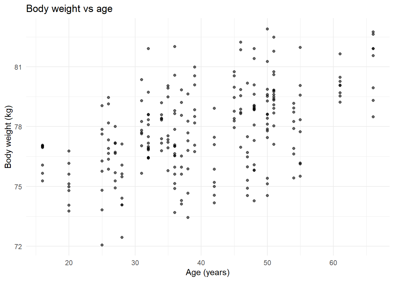
The linear regression model indicates that body weight is significantly associated with time, diet group, and age. Body weight decreases over time, reflecting the negative weekly trend built into the data generation process. Participants assigned to the standard diet have higher body weight compared to those on the high-fiber diet, and older participants tend to have slightly higher body weight.

# Logistic model: GI side effects as a function of body weight, diet group, and age
model_gi <- glm(
  GISideEffect ~ BodyWeight + DietGroup + Age,
  data = diet_data,
  family = binomial
)
summary(model_gi)

Call:
glm(formula = GISideEffect ~ BodyWeight + DietGroup + Age, family = binomial, 
    data = diet_data)

Coefficients:
                       Estimate Std. Error z value Pr(>|z|)
(Intercept)            -9.09259    6.50152  -1.399    0.162
BodyWeight              0.11458    0.08829   1.298    0.194
DietGroupStandard Diet  0.42843    0.32434   1.321    0.187
Age                     0.01131    0.01362   0.830    0.406

(Dispersion parameter for binomial family taken to be 1)

    Null deviance: 318.55  on 239  degrees of freedom
Residual deviance: 307.09  on 236  degrees of freedom
AIC: 315.09

Number of Fisher Scoring iterations: 4

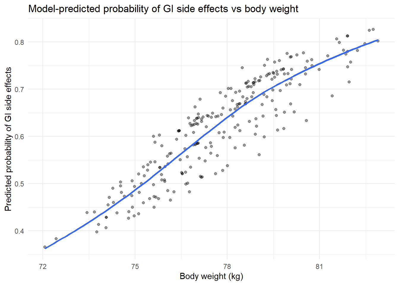
While the body weight has a positive association with the probability of gastrointestinal side effects, this association was not statistically significant. After accounting for body weight, diet group and age were not strongly associated with gastrointestinal side effects as well.

# Predicted probabilities from logistic model
diet_data$PredictedProbGI <- predict(
  model_gi,
  type = "response"
)

ggplot(diet_data,
       aes(x = BodyWeight, y = PredictedProbGI)) +
  geom_point(alpha = 0.4) +
  geom_smooth(se = FALSE) +
  labs(
    title = "Model-predicted probability of GI side effects vs body weight",
    x = "Body weight (kg)",
    y = "Predicted probability of GI side effects"
  ) +
  theme_minimal()

`geom_smooth()` using method = 'loess' and formula = 'y ~ x'

Conclusion

In this study we have a fully synthetic dataset that mimic a simple dietary intervention study. We explored how diet group, time, and age were related to body weight, and how body weight was related to gastrointestinal side effects. The analysis showed that body weight decreased over time, differed between diet groups, and increased slightly with age. The logistic regression model suggested that higher body weight was associated with a higher probability of gastrointestinal side effects, although this relationship was not statistically significant, and diet group and age did not show strong direct associations with GI side effects. Overall, this exercise demonstrates how synthetic data can be used to explore relationships between variables and to check whether simple models reflect known data-generation mechanisms.

Notes on AI use: AI tools (ChatGPT) were used in away to help clarify R syntax and structure the synthetic data generation and modeling workflow